Gnuplot

Programming in Modern Fortran

Gnuplot is a free plotting tool that can be run from the command-line or invoked by third-party applications. Despite its name, the program is not related to the GNU project. The plotting commands and the input data are read from files or stdin. The development of Gnuplot started already in 1986.

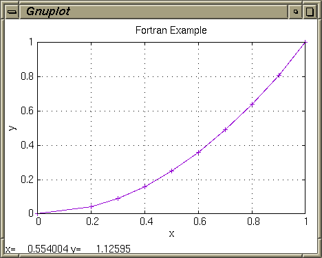
: Fig. 1: Gnuplot called from Fortran

Plots can either be displayed inside a window (fig. 1) or exported in various image formats:

Command-Line Execution
File
Anonymous Pipe
Process
Terminal Output

Command-Line Execution

The Fortran example below writes the output data to a text file data.txt, and then uses the intrinsic Fortran 2008 routine execute_command_line() to call Gnuplot. Additional Fortran modules are not required.

! example.f90
program main
    implicit none
    character(len=*), parameter :: OUT_FILE = 'data.txt' ! Output file.
    character(len=*), parameter :: PLT_FILE = 'plot.plt' ! Gnuplot file.
    integer,          parameter :: N        = 10         ! Number of values.

    integer :: i, fu
    real    :: x(N), y(N)

    x(1) = 0.0
    y(1) = 0.0

    do i = 2, N
        x(i) = 0.1 * i
        y(i) = x(i)**2
    end do

    open (action='write', file=OUT_FILE, newunit=fu, status='replace')

    do i = 1, N
        write (fu, *) x(i), y(i)
    end do

    close (fu)

    call execute_command_line('gnuplot -p ' // PLT_FILE)
end program main

The command-line argument -p lets the opened window persist. The Gnuplot commands to display the plot are stored in file plot.plt:

# plot.plt
set term x11 font "-*-helvetica-medium-r-*-*-14-*-*-*-*-*-*-*"
set title "Fortran Example"
set nokey
set grid
set xlabel "x"
set ylabel "y"
m="data.txt"
plot m using 1:2 with linespoints

The file will then be read by Gnuplot to perform the actual plotting:

$ gfortran13 -o example example.f90
$ ./example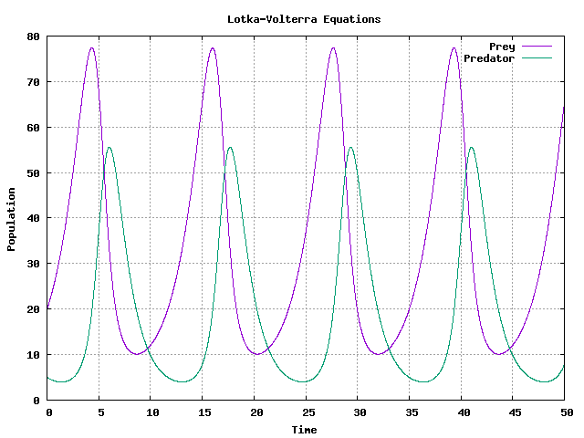

: Fig. 2: Output of Gnuplot as image file

File

We can extend the approach and configure Gnuplot to save the plot to an image file instead. The next example rk4.f90 solves the Lotka-Volterra system, a pair of non-linear ordinary differential equations which describe an ecological predator-prey model:

Lotka-Volterra ODEs

The program implements the Runge-Kutta 4th order method to solve the equations. The results are simply printed to standard output, to be piped to file, and then plotted with Gnuplot.

! rk4.f90
program main
    use, intrinsic :: iso_fortran_env, only: r8 => real64
    implicit none
    ! Point estimates for model parameters taken from:
    !     https://www.math.tamu.edu/~phoward/m442/modbasics.pdf
    real(kind=r8), parameter :: ALPHA = 0.470_r8  ! Reproduction rate of prey.
    real(kind=r8), parameter :: BETA  = 0.024_r8  ! Death rate of prey by predator.
    real(kind=r8), parameter :: DELTA = 0.023_r8  ! Reproduction rate of predator by prey.
    real(kind=r8), parameter :: GAMMA = 0.760_r8  ! Death rate of predator.

    real(kind=r8), parameter :: T_MAX = 50.0_r8   ! Max. time.
    real(kind=r8), parameter :: H     = 0.01_r8   ! Step size.
    integer,       parameter :: N     = T_MAX / H ! Number of steps.

    integer       :: i
    real(kind=r8) :: r(2)
    real(kind=r8) :: t(N), x(N), y(N)

    ! Steps.
    t = [ (H * i, i = 1, N) ]

    ! Initial prey and predator population.
    r = [ 20.0_r8, 5.0_r8 ]

    ! Solve and print results to standard output.
    do i = 1, N
        x(i) = r(1)
        y(i) = r(2)

        r = r + rk4(r, t(i), H)
        print '(3(f15.8))', t(i), x(i), y(i)
    end do
contains
    pure function f(r, t)
        !! Lotka-Volterra equations.
        real(kind=r8), intent(in) :: r(2) !! Values.
        real(kind=r8), intent(in) :: t    !! Step.

        real(kind=r8) :: f(2)
        real(kind=r8) :: u, v

        u = r(1)
        v = r(2)

        f(1) =  u * (ALPHA - BETA * v)
        f(2) = -v * (GAMMA - DELTA * u)
    end function f

    pure function rk4(r, t, h)
        !! Runge-Kutta 4th order solver for function `f(r, t)`.
        real(kind=r8), intent(in) :: r(2) !! Values.
        real(kind=r8), intent(in) :: t    !! Step.
        real(kind=r8), intent(in) :: h    !! Step size.

        real(kind=r8) :: rk4(2)
        real(kind=r8) :: k1(2), k2(2), k3(2), k4(2)

        k1 = h * f(r,            t)
        k2 = h * f(r + 0.5 * k1, t + 0.5 * h)
        k3 = h * f(r + 0.5 * k2, t + 0.5 * h)
        k4 = h * f(r + k3,       t + h)

        rk4 = (k1 + (2 * k2) + (2 * k3) + k4) / 6
    end function rk4
end program main

The Gnuplot script plot.plt sets the output format to PNG, and the file name to plot.png. The timeseries are read from file data.txt:

# plot.plt
set term png
set output "plot.png"
set title "Lotka-Volterra Equations"
set grid
set xlabel "Time"
set ylabel "Population"
plot "data.txt" using 1:2 with lines title "Prey", "data.txt" using 1:3 with lines title "Predator"

Compile the program source, execute the binary rk4, pipe the output to data.txt, and finally plot to plot.png by running the Gnuplot script plot.plt:

$ gfortran13 -o rk4 rk4.f90
$ ./rk4 > data.txt
$ gnuplot -c plot.plt

Open plot.png in an image viewer (fig. 2). We can further automate the plotting step with the help of a short shell script makeplot.sh:

#!/bin/sh

set -e

./rk4 > data.txt
gnuplot -c plot.plt

Save the script in the same directory as the binary rk4, and set execution rights:

$ chmod a+x makeplot.sh
$ ./makeplot.sh

Anonymous Pipe

Instead of transfering the output data to Gnuplot by file, we can feed plotting options and data values directly by connecting both applications with Unix pipes. The output of the Fortran program will become the input of Gnuplot.

The following example shows how to plot a shaded height map based on Perlin noise with Gnuplot (fig. 3). The Fortran program will simply print the height map to stdout. If we set the dgrid3d option followed by the correct dimensions of the matrix, Gnuplot will map a non-grid input to the internal grid format automatically. We could then output single coordinates (x, y, z) line by line instead of the matrix as a whole. Obviously, this is slower.

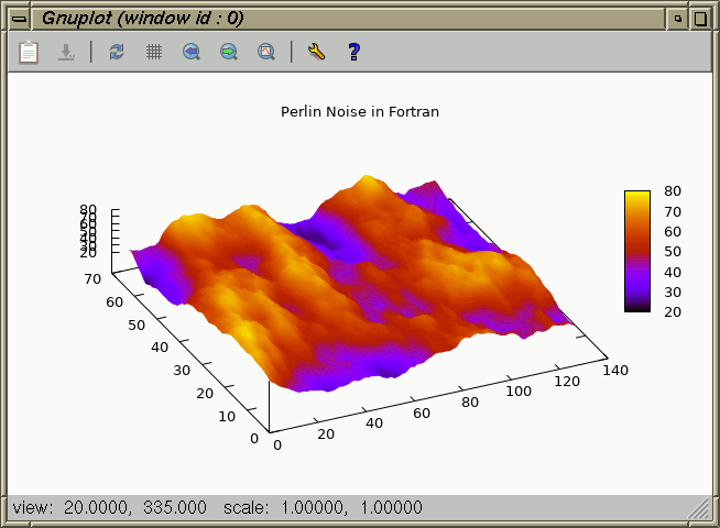
: Fig. 3: Perlin noise generated in Fortran and visualised by Gnuplot

The Fortran module perlin.f90 provides the basic Perlin noise implementation that is called by the example. Gnuplot will additionally interpolate the surface.

! matrix.f90
program main
    use :: perlin
    implicit none
    integer, parameter :: WIDTH  = 128
    integer, parameter :: HEIGHT = 64

    integer :: x, y
    real    :: r
    real    :: matrix(WIDTH, HEIGHT)

    ! Set Perlin noise seed.
    call random_seed()
    call random_number(r)
    call perlin_noise_seed(int(r * 10e6))

    ! Set Gnuplot options.
    print '(a)', 'set nokey'                           ! Disable legend.
    print '(a)', 'set cbtics scale 0'                  ! Disable colourbar tics.
    print '(a)', 'set title "Perlin Noise in Fortran"' ! Set title.
    print '(a)', 'set pm3d interpolate 2, 2'           ! Draw 3d data as colour map.
    print '(a)', 'splot "-" matrix with pm3d'          ! Plot matrix data in 3d.

    ! Calculate matrix values and print them to stdout.
    do y = 1, HEIGHT
        do x = 1, WIDTH
            matrix(x, y) = perlin_noise(real(x * .1), real(y * .1), 0.4, 8) * 100
            write (*, '(f8.5, " ")', advance='no') matrix(x, y)
        end do
        write (*, *)
    end do
end program main

The example can be compiled and executed with:

$ gfortran13 -c perlin.f90
$ gfortran13 -o matrix matrix.f90 perlin.o
$ ./matrix | gnuplot -p

We do not need to run the example each time to display the plot. Instead, redirect the output to a file first, then pipe the file contents to Gnuplot:

$ ./matrix > data.txt
$ cat data.txt | gnuplot -p

Process

On Linux and FreeBSD, Gnuplot can be executed as a sub-process, and connected to Fortran through a pipe stream, using the POSIX function popen(3). The required interface bindings to the necessary C functions are included in the fortran-unix library.

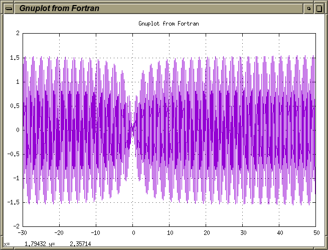
: Fig. 4: Calling Gnuplot through a subprocess on Unix

In this approach, we do not need to pipe the output of the Fortran program to Gnuplot from the shell. Instead, we open a pipe for writing, fork, invoke the shell, and execute Gnuplot in persistent mode, directly from Fortran, just by calling popen(3), fputs(3), and pclose(3).

Clone the fortran-unix repository and build the static library libfortran-unix.a:

$ git clone https://github.com/interkosmos/fortran-unix
$ cd fortran-unix/
$ make freebsd

On Linux, instead run:

$ make linux

Optionally, install the library system-wide, for example, to /opt:

$ make install PREFIX=/opt
--- Installing libfortran-unix.a to /opt/lib/ ...
--- Installing module files to /opt/include/libfortran-unix/ ...

The application has to import the module unix first. The name or path to the gnuplot(1) binary may have to be changed according to the local environment.

! process.f90
program main
    use :: unix
    implicit none
    character(len=*), parameter :: GNUPLOT = 'gnuplot' ! Name/path of Gnuplot binary.
    integer,          parameter :: N       = 800       ! Number of values.
    real,             parameter :: XSTEP   = 0.1       ! Step size.

    integer :: i
    real    :: x(N), y(N)

    ! Generate plotting data.
    do i = 1, N
        x(i) = -30 + ((i - 1) * XSTEP)
        y(i) = sin(x(i) * 20) * atan(x(i))
    end do

    ! Plot the data as line chart.
    call plot(x, y, 'Gnuplot from Fortran')
contains
    subroutine plot(x, y, title)
        !! Opens pipe to Gnuplot, writes Gnuplots settings, and plots
        !! X, Y data as line chart in an X11 window.
        real,             intent(inout) :: x(:)  !! X values.
        real,             intent(inout) :: y(:)  !! Y values.
        character(len=*), intent(in)    :: title !! Plot and window title.

        character(len=80) :: buffer
        integer           :: i, rc
        type(c_ptr)       :: ptr

        ! Create a pipe for writing, then fork, invoke the shell, and run Gnuplot.
        ptr = c_popen(GNUPLOT // c_null_char, 'w' // c_null_char)

        if (.not. c_associated(ptr)) then
            print '("Error: failed to open pipe to Gnuplot")'
            return
        end if

        ! Open persistent X11 window, set window title.
        call puts(ptr, 'set terminal x11 persist title "' // trim(title) // '"')

        call puts(ptr, 'set title "' // trim(title) // '"') ! Plot title.
        call puts(ptr, 'set grid')                          ! Enable grid.
        call puts(ptr, 'set nokey')                         ! Disable legend.
        call puts(ptr, 'plot "-" using 1:2 with lines')     ! Create line chart.

        ! Output X, Y data.
        do i = 1, size(x)
            write (buffer, '(f12.8, 1x, f12.8)') x(i), y(i)
            call puts(ptr, buffer)
        end do

        ! End plot data.
        call puts(ptr, 'e')

        ! Close the pipe.
        rc = c_pclose(ptr)
    end subroutine plot

    subroutine puts(ptr, str)
        !! Writes string to pipe, appends new line and null termination.
        type(c_ptr),      intent(in) :: ptr
        character(len=*), intent(in) :: str

        integer :: rc

        rc = c_fputs(trim(str) // c_new_line // c_null_char, ptr)
    end subroutine puts
end program main

The program has to be linked against the fortran-unix interface library. If the library is installed to /opt, compile and link with:

$ gfortran13 -I/opt/include/libfortran-unix -o process process.f90 /opt/lib/libfortran-unix.a
$ ./process

Gnuplot will run persistently as an independent process, and not terminate with the Fortran program it was called from (fig. 4).

Driver Description domterm DomTerm terminal emulator with embedded SVG dumb ASCII art for anything that prints text sixelgd Sixel using libgd and TrueType fonts sixeltek Sixel output using bitmap graphics tek40xx Tektronix 4010 and others; most TEK emulators tek410x Tektronix 4106, 4107, 4109 and 420X terminals vttek VT-like tek40xx terminal emulator: Table 1: Selection of Gnuplot’s terminal-based drivers

Driver	Description
`domterm`	DomTerm terminal emulator with embedded SVG
`dumb`	ASCII art for anything that prints text
`sixelgd`	Sixel using libgd and TrueType fonts
`sixeltek`	Sixel output using bitmap graphics
`tek40xx`	Tektronix 4010 and others; most TEK emulators
`tek410x`	Tektronix 4106, 4107, 4109 and 420X terminals
`vttek`	VT-like tek40xx terminal emulator

Terminal Output

One of the lesser known features of Gnuplot is the option to display plots directly in the terminal emulator by using one of the provided pseudo-graphics drivers. We can output a list of all supported drivers in the Gnuplot interpreter:

$ gnuplot
gnuplot> set term

Available terminal types:
       cairolatex  LaTeX picture environment using graphicx package and Cairo backend
           canvas  HTML Canvas object
              cgm  Computer Graphics Metafile
          context  ConTeXt with MetaFun (for PDF documents)
          domterm  DomTerm terminal emulator with embedded SVG
           dpu414  Seiko DPU-414 thermal printer [small medium large]
             dumb  ascii art for anything that prints text
[…]

Or, run echo "set term" | gnuplot in the terminal. The backends sixelgd and sixeltek require a Sixel-compatible terminal, such as xterm(1) or mlterm(1) on Unix (table 1). Terminal emulators which do not support the format will ignore any Sixel data. XTerm has to be run in VT340 mode to enable Sixel graphics:

$ xterm -ti vt340

Add the following lines to your ~/.Xdefaults to select the mode by default:

xterm*decTerminalID: vt340
xterm*numColorRegisters: 256

Or, start XTerm in Tektronix mode by running xterm -t instead. The environment variable TERM should be set to xterm.

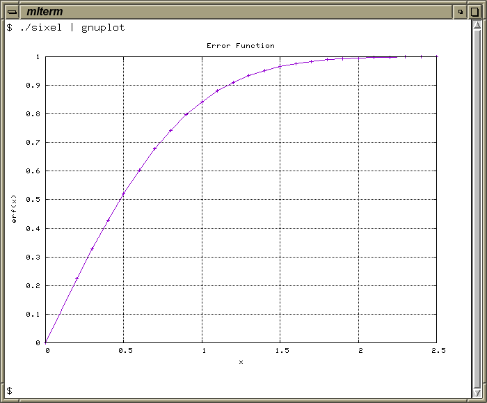
: Fig. 5: Plotting directly to mlterm(1) through the Gnuplot Sixel backend

The example program sixel.f90 prints the results of the intrinsic error function

erf(x)

and all necessary Gnuplot options to stdout. We can change the backend in parameter TERM.

! sixel.f90
program main
    implicit none
    character(len=*), parameter :: TERM   = 'sixeltek'
    character(len=*), parameter :: TITLE  = 'Error Function'
    character(len=*), parameter :: XLABEL = 'x'
    character(len=*), parameter :: YLABEL = 'erf(x)'
    integer,          parameter :: N      = 25

    real    :: x(N), y(N)
    integer :: i

    x(1) = 0.0
    y(1) = 0.0

    do i = 2, N
        x(i) = 0.1 * i
        y(i) = erf(x(i))
    end do

    print '("set term ", a)', TERM                    ! Set backend.
    print '("set nokey")'                             ! Disable legend.
    print '("set grid")'                              ! Enable grid.
    print '("set title ''", a, "''")', TITLE          ! Set plot title.
    print '("set xlabel ''", a, "''")', XLABEL        ! Set x axis label.
    print '("set ylabel ''", a, "''")', YLABEL        ! Set y axis label.
    print '("plot ''-'' using 1:2 with linespoints")' ! Plot following data as line graph.

    do i = 1, N
        print '(f12.5, ",", f12.5)', x(i), y(i)
    end do
end program main

Single quotes ' in the format specifiers have to be escaped as ''. Simply pipe the output of the program to Gnuplot. The result is shown immediately (fig. 5):

$ gfortran13 -o sixel sixel.f90
$ ./sixel | gnuplot

Optionally, we may save the Sixel image to file:

$ ./sixel | gnuplot > plot.six
$ cat plot.six

The library libsixel provides encoders and decoders for the Sixel format which can be invoked from the command-line.

Fortran Libraries

A selection of Gnuplot libraries is available for Fortran:

GNUFOR: A Fortran 90 interface for Gnuplot with data and command file output. Gnuplot is then called to run the plot script.
GNUFOR2: An interface based on GNUFOR.
Gnuplotfortran: A Fortran 95 interface that requires fortranposix.
ogpf: An object-oriented interface to Gnuplot for Fortran 2003.

References

Gnuplot: Official website

< DISLIN

[Index]

NetCDF >